Introduction

When I was in school I ran across a robot named Cubli, a research project out of ETH Zurich. This robot was actuated by a set of orthogonal inertial wheels that imparted torques on it’s cube shaped body. Using these torques, the team was able to control the robot to balance on an edge or even a corner! I’ve always wanted to make a robot like this and it sounded like a good candidate project for a reinforcement learning control policy. It also was a good introductory project to working with the Isaac Sim and Isaac Gym toolset.

Building the Simulated Cubli

Universal Robot Descriptor File (URDF)

One of the simplest ways of designing a robot to use in physics sims like Isaac is through a URDF. A URDF describes a robot with elements like Links and Joints. These connections are stored in a tree starting at a root element.

• Links described the rigid bodies of a robot

  • Links contain the visual description that is used during rendering

  • Links contain the collision description that allows the robot to touch other objects in the environment

  • Links contain inertial information

    • Center of Mass

    • Mass Value

    • Inertial Matrix

  • For mor information about URDF links, see : http://wiki.ros.org/urdf/XML/link

• Joints describe the way in which rigid bodies are connected. Each joint is a degrees of freedom the robot can move with

  • Joints have an orientation and location relative to the origin of the parent rigid Body

  • The joints used in this project are :

    • Continuous Joints. Rotation joints without a max and min angle

    • Fixed Joints. Constrains a child rigid body to the transformation of a parent rigid body.

  • For more information about URDF joints, see : http://wiki.ros.org/urdf/XML/joint

The design of my CubeBot follows the following structure.

• CubeBody

  • Continuous Joint : Inertial Wheels. (six wheels in total, one for each cube face)

    • Fixed Joint : Wheel Marker (this is just a visual element so the spinning can be observed more easily)

  • Fixed Joint : CornerBumper (eight, one per corner of the cube)

Using XML Macros (Xacro) to make URDFs easier to create

In my first iteration of the CubeBot, I created the URDF from scratch. The file tends to have a lot of repeated elements and becomes cumbersome to navigate pretty quickly. One way to mitigate this is through the use of xacro files. These files allow you to create templates for pieces of the robot and instantiate them as needed. The benifits I’ve noticed are

• The overall amount of code that needs to be written was reduced since pieces could be reused

• This helps mitigate typo bugs, and allows changes to be made much faster.

• Variables such as mass, size, color, ect can be defined in one place so you won’t need to hunt through your code and manually change every instance

• The instantiation of links and joints is in one spot which makes understanding the structure of the robot from code much easier

The URDF and Xacro files can be inspected in the github repo :

Importing into Isaac Gym and first tests

Controlling the Degrees of Freedom

The next thing to do is to verify that the robot is working as expected. I found that the best way to approach this was to modify some of the Issac Gym example codes to create an environment where the robot’s degrees of freedom could all be actuated. The original code examples come with the IsaacGym files : isaac/isaacgym/python/examples/. I found modifying the dof_control.py example to be the most convenient for testing my URDF files. To view the modified example code use the link below.

I used this part of the project to tweak the Max Torque and Max Velocity setting to make sure the CubeBot could actuate itself. I tried to keep parameters near operating parameters of commercially available brushless motors. Specifically I used Maxon: EC90 Flat 600W as a reference for the max speed and torque.

Constructing the Observation tensor

This is a good time to start constructing the observation tensor to make sure it is working like we expect it to. For this task I started with :

1. The root state tensor

   1. World Position (x,y,z)

   2. Orientation Quaternion (q1,q2,q3,q4)

   3. World Linear Velocity (x,y,z)

   4. World Angular Velocity (x,y,z)

2. DOF Velocity (Inertial Wheels[0:6])

I believe with these observations the cube should be able to learn a control policy for balancing. The velocities might need to be switch to the local frame.

We can obtain the root state tensor with the following code :

• The actor root state is unwrapped into a torch tensor. For organization we can create variables of each slices of the root state to obtain root_pos, root_ori, root_linvel and root_angvel. Each of these points to the root_states variable so updating root_pos will change root_states as well.

• root_states is located on the CPU but needs to be updated from the GPU pipeline. This can be done with a function call :

  • gym.refresh_actor_root_state_tensor(sim)

Similar to the root state, the dof state can be obtained with the following code :

• The dof state tensor contains information about all the dof in the sim. Since we only have one actor this wont be too complicated. With multiple actors we will need to keep better track of which dof belongs to which actor.

• Like the root_state, the dof_state is unwrapped to a torch tensor

• Like the root_state, the dof_state is seperated into the dof_pos and dof_vel components

• Like the root_state, the dof_state needs to be updated with a function call :

  • gym.refresh_dof_state_tensor(sim)

The action tensor

To keep things simple for now, we will be using 6 actions for the CubeBot. Each face of the bot has an inertial wheel with a DOF so each action will directly control an inertial wheel. The actions are in the range [-1, 1] and will be scaled by the MaxVelocity parameter. This allows the bot to control the target velocity of each of the inertial wheels.

First Reinforcement Learning Task

Now that we know the cube is behaving somewhat realistically, we can start modifying some of the other example code to get an environment running to teach our CubeBot. I started by modifying the CartPole example code to get this project off the ground. There are a few files we will need to edit to make sure things work correctly.

• We need to create a new VecTask for our project. The class will be called CubeBot. The names of subsequent files will be named according to this class name.

  • This file defines the parameters of the simulation and the definition of our robot

  • CubeBot.py should be in the directory training/tasks

• We need to add this new VecTask to the __init__.py file so it can be referenced by other files outside this directory

  • __init__.py should be in training/tasks

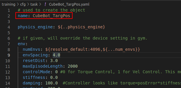
• We need to create a new configuration file called CubeBot.ymal

  • This contains parameters for setting up the environment simulation

  • This should be in the directory : training/cfg/tasks

• We need to create a new configuration file called CubeBotPPO.ymal

  • This contains the parameters used by RL_Games in there algorithm implementations

  • This should be in the directory : training/cfg/train

Most of the work we will be doing will be in the CubeBot.py : CubeBot class.

• __init__ is where we will parse the configuration data from the ymal file, define the observation tensors, and create the sim.

• The super, VecTask init called self.create_sim()

  • create_sim() will create the environments for our learning task

  • create_sim() calls _create_envs(). It is here where the assets are loaded, initial states are set, the dof_properties for the actor are set.

• compute_rewards() calls a jit script that returns rewards and the reset state for each environment.

  • A jit script will compile our python code with the TorchScript compiler so it can be run on the GPU

• compute_observations() is where we will update our observation buffer

  • In this first project, the compute_observations function is not a jit script. In later tasks we will change this to a jit script.

• reset_idx()

  • This function is responsible for resetting environments that have reached a done state.

  • The set_actor_root_state_tensor_indexed, allows us to update the state of an actor directly

  • The set_dof_state_tensor_indexed, allows us to update the state of the dof tensor.

• pre_physics_step()

  • Here we apply the actions determined by the RL network

  • This function is called in the super class, step() routine

  • After this step, the physics of the simulation are updated by 1 timestep

• post_physics_step()

  • Here the environment resets are handled first

  • We call the compute_observations function

  • We call the compute_reward function

The reward Function

The reward function is how we will direct the behavior learned by the RL agent. For this example we will simply reward the bot on each step with the Z-height of the first corner bumper on the CubeBot. This corner is highlighted in yellow in the videos.

• reward = corner_height

The RL algorithm will try to maximize the reward and thus, the cube should learn a control policy that brings the corner to the highest possible position. Ideally this requires staying in the unstable equilibrium point of balancing on one corner. There are three states I can imagine the algorithm finding.

• Laying on a face with the first corner on the top. This will result in a reward of 0.3 on each step. 0.3 is the box edge length

• Balancing on an edge with the first corner on top. This is an improvement of the above policy and would result in a reward of about 0.42 on each step.

• Balancing on a corner with the first corner on top. This should maximize the reward and result in about 0.52 reward on each step.

Initial Training Results

For this first run, the only reward parameter was the corner height. The training ran 80 million environment steps in about 20 minutes. THIS IS HUGE! This quantity of environment samples using PyBullet would have taken days! Needless to say, the Isaac Gym environment learns very fast when compared to other environments. Below is a snapshot of the reward vs. step logged in tensorboard :

It seems to have achieved it’s maximum reward fairly early, around 20M steps. The decline in performance may be from catastrophic forgetting, as the agent does better it has less examples in it’s experience buffer of ‘bad’ states. Over time it may learn policies that do not handle these states well. Lets take a look at the performance of a few of the checkpointed models. We will look at : 500k (First Saved Model), 1.5M , 10M, 20M, 50M and 82M(Last Saved Model).

Adding a second parameter to the reward

We can add parameters to the reward to shape the learned behavior. Lets try adding a penalty associated with large rotational velocities for each of the inertial wheels. Below we will take the average of the square of the wheel speeds. The wheel_speeds variable is scaled by the maximum speed resulting in a value between [-1, 1]

So how did it perform?

It seems to be able to place the first corner face up but it never learned the behavior of balancing. Maybe given more time it would learn a policy that achieves this but it might be too far outside the range of actions that this policy will randomly select.

The relative scale of rewards between the corner height and the wheel velocities might have lead to a situation where it wasn’t worth standing up because too many points would be lost spinning the wheels at a high enough velocity to stand. Lets try this again by this time we will scale the penalty by a multiplier. I’m going to use 0.5 and 0.1 and see how they compare to the previous results

As the penalty multiplier increase, the range of velocities seems to decrease. This somewhat confirms that the original wheel velocity penalty was causing the cube not to learn to stand. Below is a video showing the performance of each of the three individuals plotted above.